Advanced topics¶

Building your own X matrix¶

The X matrix in an epistasis model maps genotypes to epistatic coefficients. The rows represent the binary representation of genotypes, and the columns represent the epistatic coefficients. In a “local” epistasis model, an element in the matrix is 1 if the genotype in that element’s row has the epistatic interaction in that element’s column. Otherwise, the element is a 0 (see the example below).

If you want to generate your own X matrix, you’ll need a list of genotypes (in their binary representation) and a list of epistatic coefficients you’d like to fit. Then, you can generate X using the get_model_matrix function. Here is an example:

Input

# imports
from epistasis.matrix import get_model_matrix

# Epistasis coefficients
coefs = [
    [0],                        # Reference state
    [1], [2], [3],              # Additive coefficients
    [1, 2], [1, 3], [2,  3],    # Pairwise coefficients
    [1, 2, 3]                   # Third order coefficients
]

# List of binary coefficients
binary_genotypes = [
    '000',
    '001',
    '010',
    '100',
    '011',
    '101',
    '110',
    '111'
]

# Build X matrix
X = get_model_matrix(binary_genotypes, coefs, model_type='local')

Output

X = array([
    [1, 0, 0, 0, 0, 0, 0, 0],
    [1, 0, 0, 1, 0, 0, 0, 0],
    [1, 0, 1, 0, 0, 0, 0, 0],
    [1, 1, 0, 0, 0, 0, 0, 0],
    [1, 0, 1, 1, 0, 0, 1, 0],
    [1, 1, 0, 1, 0, 1, 0, 0],
    [1, 1, 1, 0, 1, 0, 0, 0],
    [1, 1, 1, 1, 1, 1, 1, 1]
])

Input

You can easily generate the coefficient list using a few helper functions:

from epistasis.mapping import mutations_to_sites

mutations = {
    0: ['0', '1'],
    1: ['0', '1'],
    2: ['0', '1']
}

# Same as the list above!
coefs = mutations_to_sites(order=3, mutations=mutations)

Output

coefs = [
    [0],
    [1], [2], [3],
    [1, 2], [1, 3], [2, 3],
    [1, 2, 3]
]

Write your own linear model¶

A linear, high-order epistasis model is a linear transformation of phenotypes \(\vec{P}\) (length L) to (Lth order) epistatic coefficients \(\vec{\beta}\) using the \(\mathbf{X}\) matrix described in the previous section.

\[\vec{P} = \mathbf{X} \cdot \vec{\beta}\]

In Python 3, this looks like:

from epistasis.matrix import get_model_matrix

# See the section above to get `coefs`
coefs = [
    [0],
    [1], [2], [3],
    [1, 2], [1, 3], [2, 3],
    [1, 2, 3]
]

# Numerical values for each coefficient
beta = [
    1.0,
    0.2, 0.3, 0.1,
    0.1, 0.05, 0.01,
    0.05
]

# Build the X matrix
X = get_model_matrix(binary_genotypes, coefs, model_type='local')

# Do the dot product
phenotypes = X @ beta

To compute linear epistatic coefficients from phenotypes, take the inverse of the equation above:

\[\vec{\beta} = \mathbf{X^{-1}} \cdot \vec{P}\]

In Python 3, this looks like:

import numpy as np
from epistasis.matrix import get_model_matrix

# See the section above to get `coefs`
coefs = [
    [0],
    [1], [2], [3],
    [1, 2], [1, 3], [2, 3],
    [1, 2, 3]
]

# Binary genotypes
binary_genotypes = ['000','001','010','100','011','101','110', '111']

# Quantitative phenotype values.
phenotypes = [1, 1.1, 1.2, 1.2, 1.3, 1.5, 1.7, 1.8]

# Build the X matrix
X = get_model_matrix(binary_genotypes, coefs, model_type='local')

# Take the inverse
X_inv = np.inv(X)

# Do the dot product
beta = X_inv @ phenotypes

Setting bounds on nonlinear fits¶

All nonlinear epistasis models use lmfit to estimate a nonlinear scale in an arbitrary genotype-phenotype map. Each model creates lmfit.Parameter objects for each parameter in the input function and contains them in the parameters attribute as lmfit.Parameters object. Thus, you can set the bounds, initial guesses, etc. on the parameters following lmfit’s API. The model, then, minimizes the squared residuals using the lmfit.minimize function. The results are stored in the Nonlinear object.

In the example below, we use a EpistasisPowerTransform to demonstrate how to access the lmfit API.

# Import a nonlinear model (this case, Power transform)
from epistasis.models import NonlinearPowerTransform

model = NonlinearPowerTransform(order=1)
model.parameters['lmbda'].set(value=1, min=0, max=10)
model.parameters['A'].set(value=10, min=0, max=100)

model.fit()

Access information about the minimizer results using the Nonlinear attribute.

# Pretty print the results!
model.Nonlinear.params.pretty_print()

Large genotype-phenotype maps¶

We have not tested the epistasis package on large genotype-phenotype maps (>5000 genotypes). In principle, it should be no problem as long as you have the resources (i.e. tons of RAM and time). However, it’s possible there may be issues with convergence and numerical rounding for these large spaces.

Reach out!¶

If you have a large dataset, please get in touch! We’d love to hear from you. Feel free to try cranking our models on your large dataset and let us know if you run into issues.

My nonlinear fit is slow and does not converge.¶

Try fitting the scale of your map using a fraction of your data. We’ve found that you can typically estimate the nonlinear scale of a genotype-phenotype map from a small fraction of the genotypes. Choose a random subset of your data and fit it using a first order nonlinear model. Then use that model to linearize all your phenotype

from gpmap import GenotypePhenotypeMap
from epistasis.models import (EpistasisPowerTransform,
                              EpistasisLinearRegression)

# Load data.
gpm = GenotypePhenotypeMap.read_csv('data.csv')

# Subset the data
data_subset = gpm.data.sample(frac=0.5)
gpm_subset = GenotypePhenotypeMap.read_dataframe(data_subset)

# Fit the subset
nonlinear = EpistasisPowerTransform(order=1, lmbda=1, A=0, B=0)
nonlinear.add_gpm(gpm_subset).fit()

# Linearize the original phenotypes to estimate epistasis.
#
# Note: power transform calculate the geometric mean of the additive
# phenotypes, so we need to pass those phenotypes to the reverse transform.
padd = nonlinear.Additive.predict(X='fit')
linear_phenotypes = nonlinear.reverse(gpm.phenotypes,
                                      *nonlinear.parameters.values(),
                                      data=padd)

# Change phenotypes (note this changes the original dataframe)
gpm.data.phenotypes = linear_phenotypes
model = EpistasisLinearRegression(order=10)
model.add_gpm(gpm)

# Fit the model
model.fit()

Estimating model uncertainty¶

The epistasis package includes a sampling module for estimating uncertainty in all coefficients in (Non)linear epistasis models. It follows a Bayesian approach, and uses the emcee python package to approximate the posterior distributions for each coefficient.

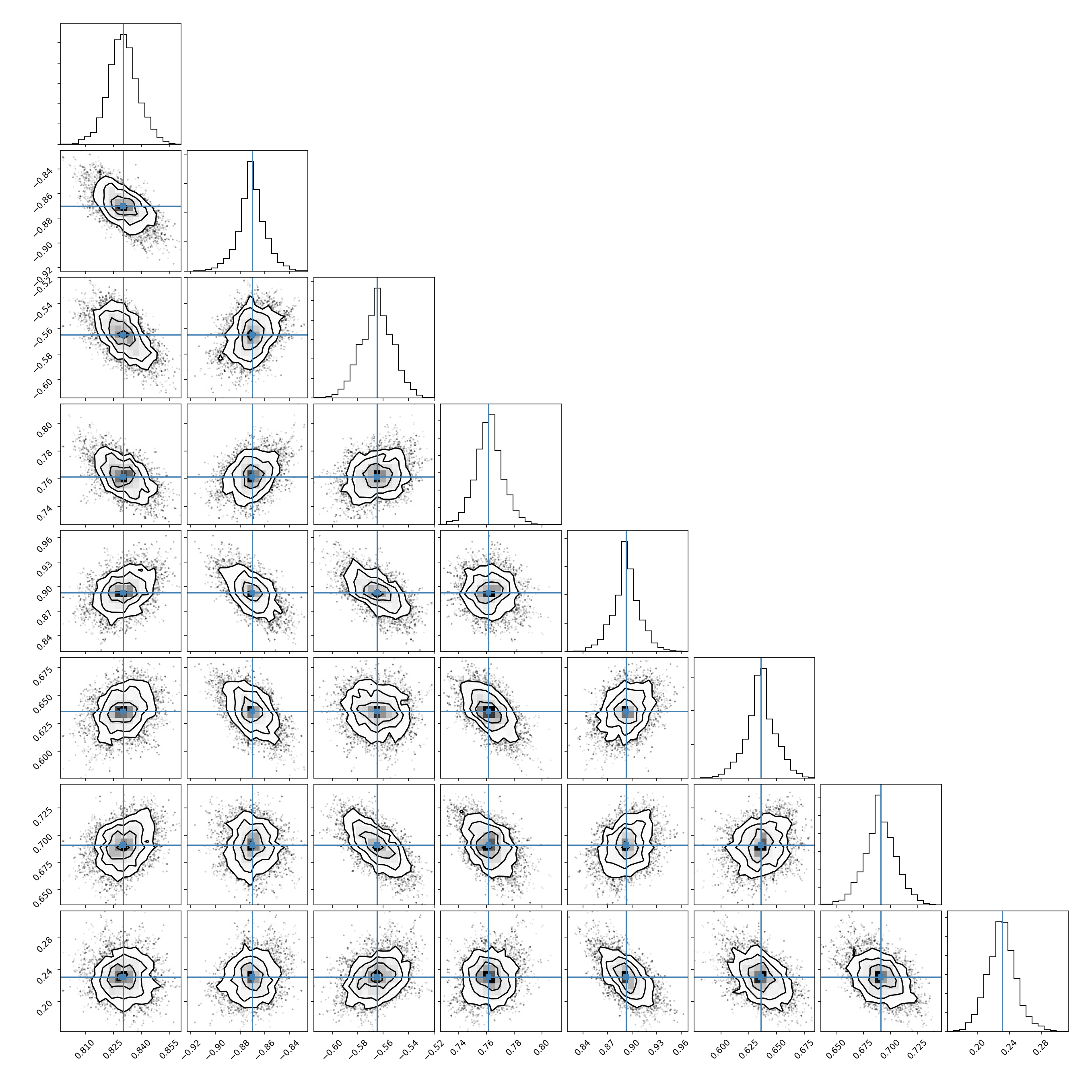
Basic example¶

Use the BayesianSampler object to sample your epistasis model. The sampler stores an MCMC chain

(The plot below was created using the corner package.)

# Imports
import matplotlib.pyplot as plt
import numpy as np
import corner

from epistasis.simulate import LinearSimulation
from epistasis.models import EpistasisLinearRegression
from epistasis.sampling.bayesian import BayesianSampler

# Create a simulated genotype-phenotype map with epistasis.
sim = LinearSimulation.from_length(3, model_type="local")
sim.set_coefs_order(3)
sim.set_coefs_random((-1,1))
sim.set_stdeviations([0.01])

# Initialize an epistasis model and fit a ML model.
model = EpistasisLinearRegression(order=3, model_type="local")
model.add_gpm(sim)
model.fit()

# Initialize a sampler.
sampler = BayesianSampler(model)
samples, rstate = sampler.sample(500)

# Plot the Posterior
fig = corner.corner(samples, truths=sim.epistasis.values)

../_images/bayes-estimate-uncertainty.png

Defining a prior¶

The default prior for a BayesianSampler is a flat prior (BayesianSampler.lnprior() returns a log-prior equal to 0). To set your own prior, define your own function that called lnprior that returns a log prior for a set of coefs and reset the BayesianSampler static method:

def lnprior(coefs):
    # Set bound on the first coefficient.
    if coefs[0] < 0:
        return -np.inf
    return 0

# Apply to fitter from above
fitter.lnprior = lnprior